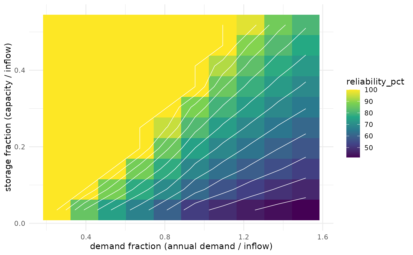
Dimensionless design curve — rh_plot_design

Re-expresses a demand x capacity rh_grid() in non-dimensional terms so the chart is transferable across sites (after Fewkes): demand becomes the demand fraction (annual demand / annual inflow) and capacity becomes the storage fraction (capacity / annual inflow). Filled by a performance metric with iso-performance contours.

Usage

rh_plot_design_curve(
  grid,
  annual_inflow,
  period_days = 365,
  metric = NULL,
  contours = TRUE,
  breaks = NULL
)

Arguments

grid: A data frame from rh_grid() varying "demand" and "capacity".
annual_inflow: Mean annual captured volume (m3), e.g. sum(rh_available_volume(precip, area, runoff, efficiency)) / n_years.
period_days: Days per year used to annualise demand. Default 365.
metric, contours, breaks: As in rh_plot_tradeoff().

Value

A ggplot2 object.

Examples

area <- 4170
n_years <- length(unique(format(precip_pi$date, "%Y")))
inflow <- sum(rh_available_volume(precip_pi$value, area, 0.85, 1)) / n_years
g <- rh_grid(precip_pi$value, base = list(area = area, runoff = 0.85, efficiency = 1),
             x = "demand", x_values = seq(2, 12, length.out = 10),
             y = "capacity", y_values = seq(100, 1500, length.out = 10),
             metrics = "reliability_pct",
             dates = precip_pi$date, climatology = TRUE)
if (requireNamespace("ggplot2", quietly = TRUE)) {
  rh_plot_design_curve(g, annual_inflow = inflow)
}